
Have you heard the news? Excel has a new FILTER function, and this isn’t your momma’s Instagram filter. If you want to be able to quickly #filter your data in Excel, you’ll want to learn this trick!
The FILTER function has three arguments: array, include, and if_empty. Array is the range of data that you are filtering, include is the criteria that you want to filter on, and the if_empty argument is a default value that the filter function will return if no values within your data array meet your criteria.
Check out the table above for an example. We’ve got sales data by rep, sales amount, and region - but let’s say we want a snapshot of only Dua Lupa sales. Instead of adding sort and filter toggles and manually filtering the data, we can use our new FILTER function! Start by inserting the FILTER function (=FILTER) and selecting the sales data as the array argument. Next we need to enter the criteria we want to apply to the data to determine which values are returned as the include argument. In this case, we’ll set the representative’s name column equal to the representative we want to filter on (cell G2, in this case!). Upon entering, the function will return all rows where the representative equals Dua Lupa. 🔥
Here’s the best part: this function is dynamic, so it automatically updates the results if any of the arguments change. For example, say we want to filter based on Bill Bates' sales, rather than Dua Lupa’s. All we need to do is update the representative to “Bill Bates” and the filter function will automatically update to pull Bill’s sales and region.
Have you tried the filter function yet? Give it a go, and let me know what you think!